Graphene on h-BN (Stacking Energy and Band Gap)

1. Introduction

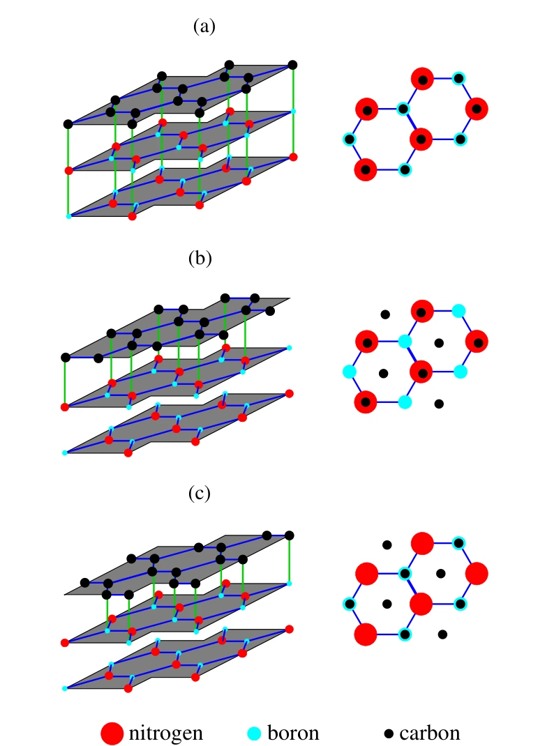
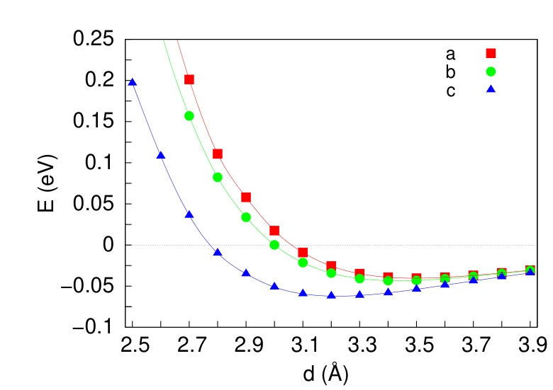
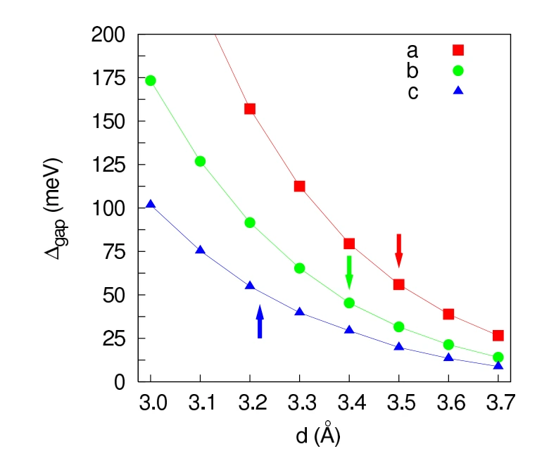
This tutorial calculates the total energy and band structure of graphene on four layers of h-BN for the three stackings (a), (b) and (c) of the structure tutorial, over a list of graphene–h-BN distances, reproducing Fig. 2 (total energy vs distance and the equilibrium distances), Fig. 3 (bands and density of states of (c) at its equilibrium distance, gap at K) and Fig. 4 (gap at K vs distance) of the following manuscript.

Manuscript

Gianluca Giovannetti, Petr A. Khomyakov, Geert Brocks, Paul J. Kelly and Jeroen van den Brink Substrate-induced band gap in graphene on hexagonal boron nitride: Ab initio density functional calculations Physical Review B 76, 073103 (2007) DOI: 10.1103/PhysRevB.76.073103 ¹

2. Prerequisites

Run the structure creation tutorial first. Its interface_2d_2d_boron_nitride_graphene.ipynb notebook creates and names the materials this notebook loads, for example Gr/hBN (c) d3.10. The defaults build stacking (c) at 3.1, 3.2 and 3.3 Å. The paper's full set is described in Customization options.

3. Workflow overview

The notebook runs the Standata band_structure_dos.json workflow once per material. It chains pw_scf (total energy), pw_bands (band structure), pw_nscf and projwfc (density of states).

The sheets are rigid and the workflow includes no relaxation step, as in the paper. The jobs run one at a time, and a re-run finds each finished job by its material and workflow name and reuses it.

4. Calculation parameters

Cell 1.2 sets the stackings, the distances, the cluster and the workflow name:

from datetime import datetime
from mat3ra.ide.compute import QueueName

ORGANIZATION_NAME = None  # set to your organization name (full or partial); otherwise, your default one is used
FOLDER = "./uploads"

# Giovannetti et al. 2007 compute all three stackings at every distance 2.5–3.9 Å; the defaults run
# stacking (c) at three distances around its minimum. Uncomment entries to compute more
# (one job per stacking × distance, ~25 min each on queue D with two cores).
STACKINGS = [
    "c",
    # "a",
    # "b",
]
DISTANCES = [
    3.1, 3.2, 3.3,
    # 2.5, 2.6, 2.7, 2.8, 2.9, 3.0, 3.4, 3.5, 3.6, 3.7, 3.8, 3.9,
]
MATERIAL_NAME = "Gr/hBN ({stacking}) d{distance:.2f}"  # as saved by the structure notebook

WORKFLOW_SEARCH_TERM = "band_structure_dos.json"
MY_WORKFLOW_NAME = "Band Structure + DOS"
APPLICATION_NAME = "espresso"

CLUSTER_NAME = "001"  # specify full or partial name i.e. "cluster-001" to select
QUEUE_NAME = QueueName.D
PPN = 2
TIME_LIMIT = "04:00:00"

timestamp = datetime.now().strftime("%Y-%m-%d %H:%M")
POLL_INTERVAL = 60  # seconds

Cell 1.3 sets the DFT parameters:

MODEL_SUBTYPE = "lda"
FUNCTIONAL = "pz"  # Giovannetti et al. 2007 use LDA: GGA gives essentially no interlayer binding
PSEUDOPOTENTIAL_TYPE = "us"  # GBRV ultrasoft, the only LDA family the platform publishes for B, C and N
ECUTWFC = 40  # Ry, GBRV's tested cutoff; the paper's 600 eV is a VASP number
ECUTRHO = 200  # Ry, GBRV's tested charge-density cutoff

KGRID = [36, 36, 1]  # Giovannetti et al. 2007; a multiple of 3 keeps K on the mesh
OCCUPATIONS_SETTINGS = {"occupations": "tetrahedra"}  # the paper's tetrahedron method
# eamp = 0: the sawtooth is the dipole correction only, no external field
DIPOLE_SETTINGS = {"control": {"tefield": True, "dipfield": True}, "system": {"edir": 3, "eamp": 0.0, "eopreg": 0.05}}
KPATH_STEPS = 100
MODEL_TAG = (f"{FUNCTIONAL}-{PSEUDOPOTENTIAL_TYPE} {ECUTWFC}-{ECUTRHO}Ry k{KGRID[0]} p{KPATH_STEPS} "
             f"{OCCUPATIONS_SETTINGS['occupations']} eamp{DIPOLE_SETTINGS['system']['eamp']}")

SCF_UNIT = "pw_scf"
NSCF_UNIT = "pw_nscf"
BANDS_UNIT = "pw_bands"
NUMBER_OF_OCCUPIED_BANDS = 20  # 40 valence electrons: C 4×2, B 3×4, N 5×4

KPATH = [
    {"point": "Γ", "steps": KPATH_STEPS},
    {"point": "K", "steps": KPATH_STEPS},
    {"point": "M", "steps": KPATH_STEPS},
    {"point": "Γ", "steps": 1},
]

VELOCITY_FIT_RANGE = (3, 8)  # path points from K used for the ħv fit
ZOOM_POINTS = 12  # path points each side of K in the zoom
ZOOM_WINDOW = 0.5  # eV each side of the band edges

paper	this notebook
LDA	LDA
VASP, plane waves, 600 eV	GBRV ultrasoft, 40/200 Ry
36×36×1	36×36×1
tetrahedron	tetrahedron (scf, nscf)
dipole correction	dipole correction (tefield, dipfield, edir = 3, eamp = 0, no external field)
4 h-BN layers at 3.24 Å	4 h-BN layers at 3.24 Å
a = 2.445 Å	a = 2.445 Å
vacuum 12–15 Å	vacuum 15 Å
rigid sheets	rigid sheets

5. Step-by-step instructions

5.1. Open the notebook

Navigate to the API examples repository and open:

other/materials_designer/specific_examples/interface_2d_2d_boron_nitride_graphene_SIMULATION.ipynb

5.2. Configure parameters

In cell 1.2, set ORGANIZATION_NAME to the account's organization, and STACKINGS and DISTANCES to the same lists as in the structure notebook. Cell 1.3 keeps the paper's settings.

5.3. Run the notebook

Select Run > Run All. The notebook authenticates with the platform (section 2), loads the materials by name, prints their provenance and saves them to the platform (section 3), configures one workflow per material (section 4), creates the compute configuration (section 5) and submits the jobs one at a time (section 6). Each ten-atom job takes about 16 minutes on queue D with two cores, so the full set runs overnight. Section 7 retrieves the total energies, gaps and plots, and section 8 prints the comparison with the paper.

5.4. Re-run the notebook

A re-run finds the finished jobs by material and workflow name and reuses them rather than resubmitting.

6. Expected results

The paper's values and the values measured by the notebook:

quantity	paper	this notebook	deviation
equilibrium distance (a)	3.50 Å	computed when "a" / "b" and the other distances are uncommented
equilibrium distance (b)	3.40 Å	computed when "a" / "b" and the other distances are uncommented
equilibrium distance (c)	3.22 Å	3.232 Å	+0.4 %
gap at K at the equilibrium distance (a)	56 meV	computed when "a" / "b" and the other distances are uncommented
gap at K at the equilibrium distance (b)	46 meV	computed when "a" / "b" and the other distances are uncommented
gap at K at the equilibrium distance (c)	53 meV	50.1 meV	−5 %
h-BN gap at K	4.7 eV	4.73 eV	+1 %
effective mass at K (c)	4.7·10⁻³ mₑ	6.7·10⁻³ mₑ	+43 %
E(c) < E(b) < E(a) at every distance	yes	computed when "a" / "b" and the other distances are uncommented

Gap at K at 3.1 / 3.2 / 3.3 Å: 75.2 / 55.0 / 39.8 meV (Fig. 4, curve (c)).

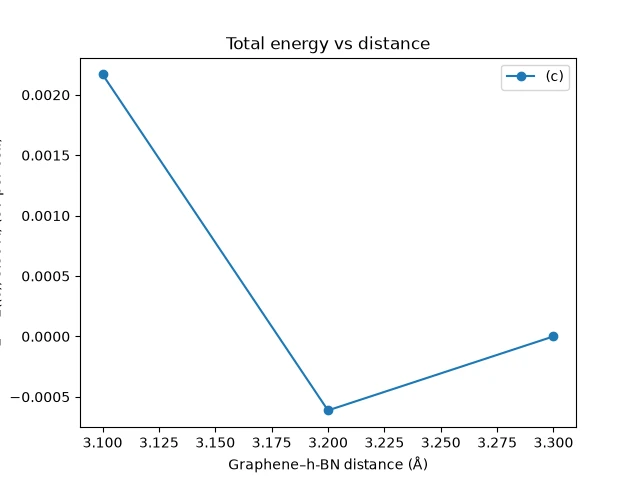
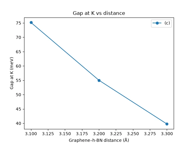
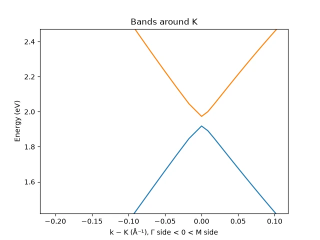
The notebook plots the total energy and the gap at K against the distance for each stacking (the paper's Fig. 2 and Fig. 4) and, for (c) at its equilibrium distance, the bands, the density of states and a zoom around K (Fig. 3).

7. Customization options

DISTANCES and STACKINGS select the materials; they must match the lists in the structure notebook. KGRID and KPATH_STEPS control the k-point sampling of the SCF/NSCF grid and the band-structure path; ECUTWFC and ECUTRHO set the plane-wave cutoffs. MODEL_TAG is built from these settings and is part of every workflow's name, so changing any of them creates new jobs rather than reusing the ones already run.

The paper's full set (three stackings × 2.5–3.9 Å) is obtained by uncommenting the STACKINGS and DISTANCES entries in both notebooks, one job per entry pair, about 25 minutes each on queue D.

8. Troubleshooting

8.1. Material not found

ValueError: No material named … means the structure notebook has not been run, or the stackings and distances do not match those of the structure notebook. Run the structure tutorial first; the names must match those the structure notebook saves.

9. Interactive JupyterLite notebook

⛶ Full Screen

10. References

---

1. Gianluca Giovannetti, Petr A. Khomyakov, Geert Brocks, Paul J. Kelly, and Jeroen van den Brink. Substrate-induced band gap in graphene on hexagonal boron nitride: ab initio density functional calculations. Physical Review B, 76:073103, 2007. doi:10.1103/PhysRevB.76.073103. ↩